Scaling Document Retrieval with Ray Data

Enhance content-based search capabilities using Ray Data's scalability and efficiency. Scale up embedding generation and hosting vector databases with Ray.

! pip install chromadb==0.4.6

import uuid
from pathlib import Path
from time import sleep

import chromadb
import numpy as np
import openai
import pinecone
import ray
from InstructorEmbedding import INSTRUCTOR
from ray import serve

Scaling document retrieval with Ray

Roadmap to scaling content-based search with Ray

1. Terminology and concepts
2. Motivation for embeddings, vector databases, and indexing
3. Getting started with vector databases via cloud services
4. Scaling up embedding generation with Ray
5. Hosting vector databases and scaling them with Ray

Much of the power of LLM-based apps comes from the “zero-shot” capabilities of the models – the ability of powerful LLMs to successfully use data, tools, and goals that they weren’t specifically trained on.

The most common way of providing new data, tools or goals is via prompt engineering or placing relevant information in the prompt.

Context window

LLMs have a limit to the size of the prompt they can work with – this size or space is a called the “context window” and has historically been limited by the model architecture or processing cost.

Document retrieval

In order to provide the most relevant bits of information to the LLM within a finite context window, we typically use one or more data sources to select relevant records (based on the prompt) out of the large pool of information we have.

Although there is a lot of research on expanding the context window to very large or even unlimited sizes, it will probably remain effective (with the currrent generation of models) to select specific responsive data and feed that to the model in order to get the best results.

Retrieval Augmented Generation (RAG)

RAG is the shorthand for this pattern: using generative models to produce output, but improving or guiding that output by placing relevant information in the prompt.

Databases

Any data store can be used for RAG applications – and in many cases it’s useful to have multiple databases …

… but almost all RAG applications rely on embeddings in a vector database in addition to other sources.

Why? Let’s see:

Here is our toy text-matching database

database = {
    'Monkeylanguage LLC' : ['Juan Williams is the CEO', 'Linda Johnson is the CFO', 'Robert Jordan is the CTO', 'Aileen Xin is Engineering Lead'],
    'FurryRobot Corp' : ['Ana Gonzalez is the CEO', 'Corwin Hall is the CFO', 'FurryRobot employs no technical staff', 'All tech is produced by AI'],
    'LangMagic Inc' : ["Steve Jobs' ghost fulfills all roles in the company"]
}

def lookup(prompt, database):
    for k in database.keys():
        if k in prompt:
            return database[k]

lookup("Tell me about Monkeylanguage LLC", database)

The problem – for empowering LLM apps – is that traditional databases don’t capture semantics

type(lookup("Tell me about the companies' top leadership", database))

Note that the problem illustrated here is not a consequence of our primitive datastore: even a full-featured SQL, document, or key-value database with full text-matching capabilities would not “realize” that top leadership refers to CEOs or C-suite roles. This key information is not a formal relationships, but a semantic relationship that lives in the world of natural language usage patterns

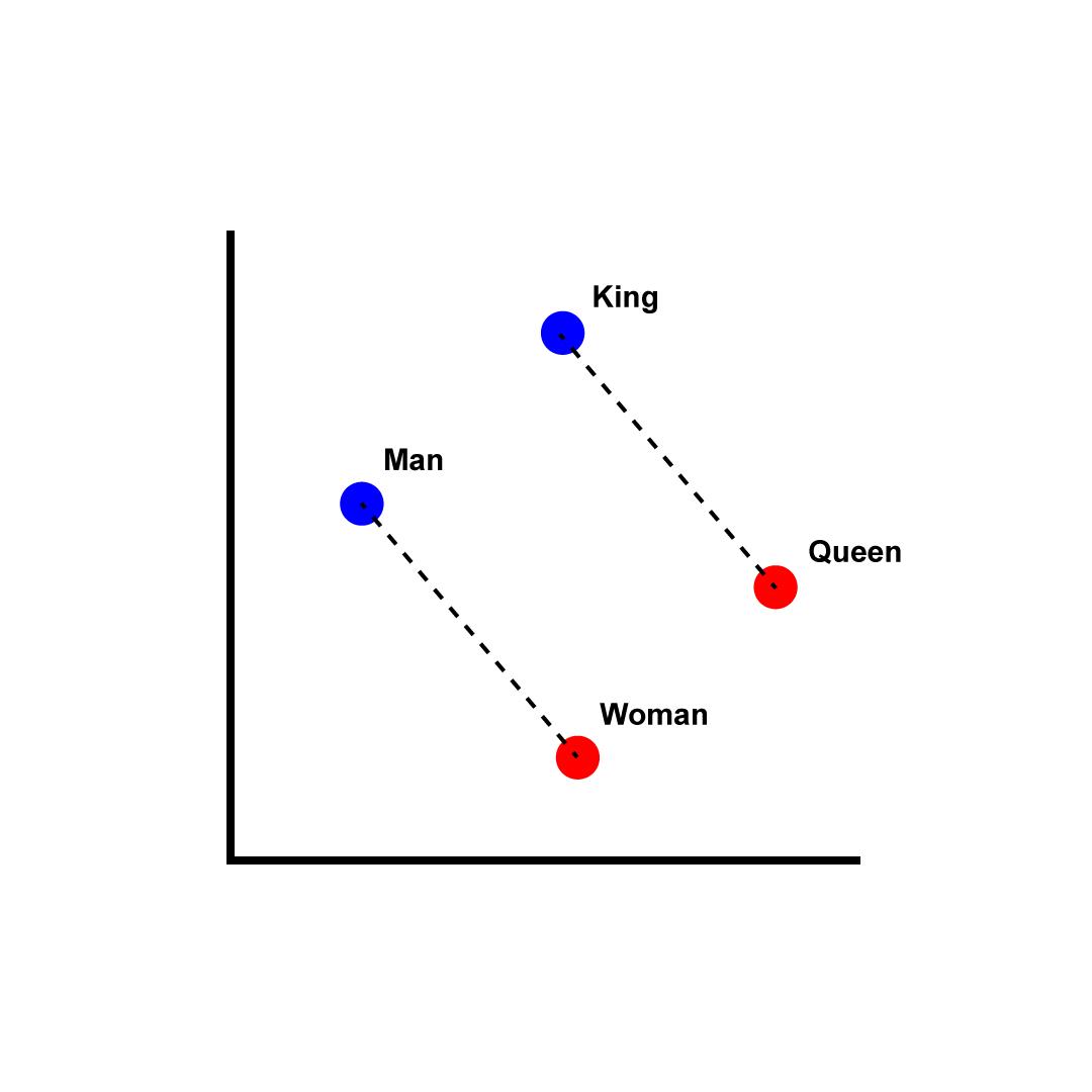
After many decades of researchers trying to solve this problem “the hard way,” we discovered the easy way: we can use simple deep-learning techniques to convert natural language into a mathematical representation that captures usage-based semantic relationships: embeddings.

The most famous models in this area (though a bit dated) are https://en.wikipedia.org/wiki/Word2vec … for a very accessible explanation see http://jalammar.github.io/illustrated-word2vec/

We can see embeddings in action using OpenAI’s models and embedding API

openaikey = Path('openaikey.txt').read_text()
openai.api_base = 'https://api.openai.com/v1'
openai.api_key = openaikey

items = sum(database.values(), [])

items

def get_embedding(text, model="text-embedding-ada-002"):
    text = text.replace("\n", " ")
    return openai.Embedding.create(input = [text], model=model)['data'][0]['embedding']

vecs = [get_embedding(item) for item in items]

arr = np.array(vecs)
arr.shape

Each of our input “documents” has been turned into a high-dimensional vector based on the prior training of the model.

Let’s see if the embeddings capture the relationships we are looking for.

We’ll make a vector representing our search

search = get_embedding("find technical leadership")

search_vec = np.array(search)

search_vec.shape

Now we’ll find the closest vectors from our original dataset based on brute-force Euclidean distance

np.sum(np.square(search_vec - arr), axis=1)

matches = np.argsort(np.sum(np.square(search_vec - arr), axis=1))
matches

print([items[i] for i in matches[:3]])

Although we can see the principles at work here, searching and indexing vectors at scale is a challenging problem, which motivates the use of dedicated vector databases. Before we look at vector stores, though, consider the task of generating embeddings.

Using a hosted model like OpenAI is easy, but

• requires sending all of our documents – which may be confidental or protected personal information – through OpenAI’s system
• incurs costs that may be hard to manage
• limits our control of the process

For production systems using senstive data, we likely want to generate the embeddings ourselves.

There are many open models that generate good embeddings.

One of the most powerful and useful is the Instructor model from Hong Kong University’s NLP group, because it allows for instruction-based finetuning: you can tell it what you’re trying to accomplish and it can generate embeddings tailored to your needs by combining your instructions with its pretraining.

Our main demo won’t feature custom instructions, but you can try instructing the model in optional lab activities.

model = INSTRUCTOR('hkunlp/instructor-large')

vectors = model.encode(items)

vectors.shape

This model is producing 768-dimension vectors

vec_dim = vectors.shape[1]
vec_dim

Now we can create high quality embeddings on our own – without sending our raw data to another company.

Let’s look at the vector storage and lookup component, both remote and local, and then we’ll look at scaling these elements in our own systems.

Indexed and approximate search

To effectively search large collections of vectors, we have a few options that let us trade off accuracy for speed. There are also a number of similarity metrics we might use.

Vector databases are systems specifically designed to support these tasks and options.

We can get started with a quick demo using a cloud service, similar to how we used OpenAI to quickly get started with embeddings. Pinecone offers a free but limited starter tier.

pineconekey = Path('pinecone.txt').read_text()

pinecone.init(api_key=pineconekey, environment="gcp-starter")

try:
    pinecone.delete_index("demo")
except pinecone.core.client.exceptions.NotFoundException:
    pass # no index / first run

pinecone.create_index("demo", dimension=vec_dim, metric="euclidean")

index = pinecone.Index("demo")

For each document, we’ll insert an id as well as a vector. We can use the id later to find the original document.

index.upsert( (str(i), vectors[i, :].tolist()) for i in range(len(items)) )

Note there is some eventual-consistency patterns involved in some parts of Pinecone, so you may not see your new vectors in the stats immediately

while total_vector_count := index.describe_index_stats()['total_vector_count'] < 9:
    sleep(1)

index.describe_index_stats()

Let’s try our tech leadership search

search = model.encode("Technical leadership")

results = index.query(
  vector=search.tolist(),
  top_k=3,
)

results

[items[int(match['id'])] for match in results['matches']]

Scaling up local embeddings and local vector search

We’ve introduced embeddings and vector stores – now let’s look at scaling up while keeping our infrastructure local.

Let’s generate embeddings for a slightly larger dataset: we’ll work with the text of Jules Verne’s Around the World in 80 Days, a popular novel now in the public domain. In your own work, you might be vectorizing instruction manuals, product descriptions, or customer service history – the concepts are the same.

We’ll start by splitting the text into paragraph-length chunks

The art of chunking: Do we always split by paragraphs? What if my data doesn’t have paragraphs? How to split your content is an important parameter to think about and “tune.” We want our chunks to represent semantic units as much as possible; to be within certain size bounds; and perhaps to reflect the structure of the data so that we can enrich our system with metadata (e.g., chapter or page numbers, product or part numbers, etc.) Sophisticated splitting algorithms exist and you should take advantage of them (https://www.pinecone.io/learn/chunking-strategies/) but spend a bit of time on design/thinking first.

text_full = Path('around.txt').read_text()
paras = text_full.split('\n')

len(paras)

Generating embeddings can be done on a CPU, but it’s slow … if we want to use our CPU-only machines, we probable want to scale out this processing

%%time

para_vecs = model.encode(paras[:50], device='cpu')

GPUs are, not suprprisinly, a lot faster … but there is still a cost

%%time

para_vecs = model.encode(paras, device='cuda:0')

para_vecs.shape

In one timing run, using a A10G GPU, we saw 3.7 ms per vector for this model and document size. In a large-scale application with 50 million document fragments, this would take about 51 hours or a bit more than two full days.

Even with GPUs, we want to scale out our embedding computation

Scaling embeddings with Ray

Ray makes it easy to scale out Python tasks like computing embeddings by

• providing the infrastructure to handle arbitrarily large datasets
• orchestrating the movement of this data from persistent storage, through memory and processing, and out to a destination
  • “destination” might be stable storage (files), a queueing system (like Kafka), a database, or something else
• efficiently managing movement of large “helper data” – like models – which are needed in various times and places during processing
• supporting pipelining or the simultaneous use of valuable compute resources for different stages of processing on different chunks of data

To take advantage of these feature, we’ll use Ray Data (https://docs.ray.io/en/releases-2.6.1/data/data.html)

We’ll start by moving our data to shared storage (e.g., a cloud storage bucket)

! cp around.txt /mnt/cluster_storage/

Create a dataset from one or more files – in this case, since our data isn’t really big, we will set parallelism to 4. (The Ray Data default parallelism heuristic is described here https://docs.ray.io/en/releases-2.6.1/data/performance-tips.html#tuning-read-parallelism)

paras_ds = ray.data.read_text("/mnt/cluster_storage/around.txt", parallelism=4)

Ray Datasets represent lazy, streaming data – similar to many other large-scale data frameworks – which improves performance but makes it a little harder to see the data, since it’s rarely all loaded up in one place and time.

We can use helper functions to inspect a small amount

paras_ds.take(5)

We will typically batch our data (also to improve performance and throughput). We can inspect a batch

sample_batch = paras_ds.take_batch()

type(sample_batch)

paras_ds.schema()

Each column in the dataset is a key/value pair in the dict. If we’re working with a batch, we’ll have vectorized types – here, numpy.ndarray of strings

sample_batch.keys()

type(sample_batch['text'])

To perform generate our emeddings, we’ll use two steps

1. Create a class that performs the embedding operation
   1. We use a class because we’ll want to hold on to a large, valuable piece of state – the embedding model itself
   2. For use with our vector databases, we’ll need unique IDs to go with each document and embedding – we’ll generate UUIDs
   3. the output from the __call__ method will be similar to the input: a dict with the column names as keys, and vectorized types for values
2. Call dataset.map_batches(...) where we connect the dataset to the processing class as well as specify resources like the number of class instances (actors) and GPUs
   1. Specify an autoscaling actor pool – to demo how Ray could autoscale to handle large, uneven workloads

class DocEmbedder:
    def __init__(self):
        self._model = INSTRUCTOR('hkunlp/instructor-large')

    def __call__(self, batch: dict[str, np.ndarray]) -> dict[str, np.ndarray]:
        inputs = batch['text']
        embeddings = self._model.encode(inputs, device='cuda:0')
        ids = np.array([uuid.uuid1().hex for i in inputs])
        return { 'doc' : inputs, 'vec' : embeddings, 'id' : ids }

vecs = paras_ds.map_batches(DocEmbedder, compute=ray.data.ActorPoolStrategy(min_size=2, max_size=8), num_gpus=0.125, batch_size=64)

Since datasets are lazy and streaming, we need to specifically ask to pull some data through to test it

vecs.take_batch()

The processing appears to work as intended.

Before we run it over the whole dataset, we need to think about where we want the data to go…

• We can’t “keep it in memory” since the whole idea of a large-scale processing framework is that our data size » memory size
• We could write to a file system if we want it for later
• Ideally, since the next step of our process is to load the vectors into a vector store and the docs into either a vector store or some other type of database, we should do something like dataset.to_my_vector_db(...)
  • As the vector database landscape settles, expect this sort of functionality to appear, similar to the existing .write_mongo
• We could also
  • convert to Dask, Mars, Modin, Arrow refs, or NumPy refs … and then use a library to write those
  • write our own datasource (consumer)

For today’s demo, we won’t build that part; we’ll collect NumPy refs: a Python list of object references (futures) to dicts with NumPy arrays holding our data

Let’s generate those object refs and take a look

numpy_refs = vecs.to_numpy_refs()

numpy_refs

To retrieve the Python objects that correspond to the references in the list, we use ray.get

ray.get(numpy_refs[0]).keys()

We can check that the values in the dict are NumPy arrays

type(ray.get(numpy_refs[0])['doc'])

Since our data isn’t that large, and we’re not demonstrating parallel writes into our vector store here, we can collect the chunks represented by object refs and stack them into single NumPy arrays

dicts = ray.get(numpy_refs)

vecs = np.vstack([d['vec'] for d in dicts])
ids = np.hstack([d['id'] for d in dicts])
docs = np.hstack([d['doc'] for d in dicts])

Let’s load up all of our vectors into our Pinecone vector database and verify that semantic search is working

texts = dict(zip(ids, docs))

count = len(ids)

index.upsert([(i, v.tolist()) for (i, v) in zip(ids, vecs)], None, 100, True)

Note that due to eventual consistency semantive in Pinecone, our vectors may not be immediately available

while total_vector_count := index.describe_index_stats()['total_vector_count'] < 1000:
    sleep(1)

Using circumlocutions, we can check that queries match targets even when the words are different

utah_query_vec = model.encode("Describe the body of water in Utah").tolist()

results = index.query(
  vector=utah_query_vec,
  top_k=3,
)

results

And we use the texts dict to look up the docs from the returned IDs. Note that some vector DBs can also store the documents. Or you can use your favority (or organization-mandated) datastore to track these, as they are just an ID and a string.

[texts[match['id']] for match in results['matches']]

Local vector stores

So far we’ve scaled our embedding processing with Ray and we’ve gotten started on vector databases quickly and easily using Pinecone in the cloud.

But for many of the same reasons we might prefer hosting our own embedding models instead of using a cloud service, we may want or need to run our own vector stores.

Luckily, there are many great, open-source vector databases which we can run locally. Some, like ChromaDB, offer open local versions and cloud service options. We’ll run Chroma locally and see how we can scale up to handle production query volumes.

First, we’ll introduce ChromaDB in a minimal in-memory form so that we can see the prorgamming pattern.

chroma_client = chromadb.Client()

collection = chroma_client.get_or_create_collection(name="my_text_chunks")

Insert the vectors, documents, and IDs

Note that Chroma can also accept arbitrary metadata dictionaries for each document, which you can then use in your queries (along with semantic similarity) and see in results. Metadata allows you to easily add powerful features like “search only in chapter 3” or “cite source URLs for data returned”

collection.upsert(
    embeddings=vecs.tolist(),
    documents=docs.tolist(),
    ids=ids.tolist()
)

See if we can learn about the Great Salt Lake

results = collection.query(
    query_embeddings=[utah_query_vec],
    n_results=3
)

results

Scaling queries with Chroma

Now that we have the basics of Chroma down, let’s look at scaling to large datasets.

Fully scalable databases are a complex topic with tradeoffs, and we’ll talk about those tradeoffs later.

For this example, we’ll focus on scaling the read path – a common OLAP pattern where we design a system that can handle arbitrary load for reading/searching the database, but does not have similar scaling for writes.

We’ll implement this query capacity with Chroma by persisting database in shared storage, and then starting as many Chroma instances as we need, using the same data source.

For this example, we’ll create the database on a local NVMe disk for speed, then move it to shared storage.

chroma_client = chromadb.PersistentClient(path="/mnt/local_storage/vector_store")

collection = chroma_client.get_or_create_collection(name="persistent_text_chunks")

collection.upsert(
    embeddings=vecs.tolist(),
    documents=docs.tolist(),
    ids=ids.tolist()
)

collection.query(
    query_embeddings=[utah_query_vec],
    n_results=3
)

Now we’ll move the data to the shared storage (in this example, cloud storage) so it can be accessed from many nodes

! cp -rf /mnt/local_storage/vector_store /mnt/cluster_storage

Scalable Chroma reader service with Ray Serve

We can define a Ray Serve deployment that queries the data using Chroma. Then we can let Ray handle autoscaling from 0 … to as much compute as we need.

@serve.deployment(autoscaling_config={ "min_replicas": 4, "max_replicas": 1000 }, 
                  ray_actor_options={ "runtime_env" : { "pip": ["chromadb"] }})
class ChromaDBReader:
    def __init__(self, collection: str):        
        chroma_client = chromadb.PersistentClient(path="/mnt/cluster_storage/vector_store")
        self._coll = chroma_client.get_collection(collection)
    
    def get_response(self, query_vec, top_n):
        return self._coll.query(query_embeddings=[query_vec], n_results=top_n,)['documents']

search_handle = serve.run(ChromaDBReader.bind('persistent_text_chunks'), name='doc_search')

ray.get(search_handle.get_response.remote(utah_query_vec, 3))

Let’s try a new query …

ray.get(search_handle.get_response.remote(model.encode('bank robbery details').tolist(), 3))

And let’s make sure it works on multiple nodes:

• We should have multiple ChromaDBReader replicas
• With load balancing at work, a few requests should hit make sure multiple replicas are used
• Check the Ray dashboard cluster view to verify that queries are succeeding on multiple nodes in the cluster

for i in range(4):
    print(ray.get(search_handle.get_response.remote(model.encode('bank robbery details').tolist(), 3)))

Review: local at-scale embeddings and search

In this module, we’ve looked at the motivation for embeddings and vector databases.

We’ve talked about why we often want to run both of those services in our own infrastrucure, keeping our own data private, and allowing us to control architecture, functionality, and costs.

And we’ve seen how Ray Tasks and Ray Serve deployments make it simple to start with code and tools we’ve learned during local prototyping … and to then scale up to arbitrarily large amounts of data and compute in production.

serve.shutdown()