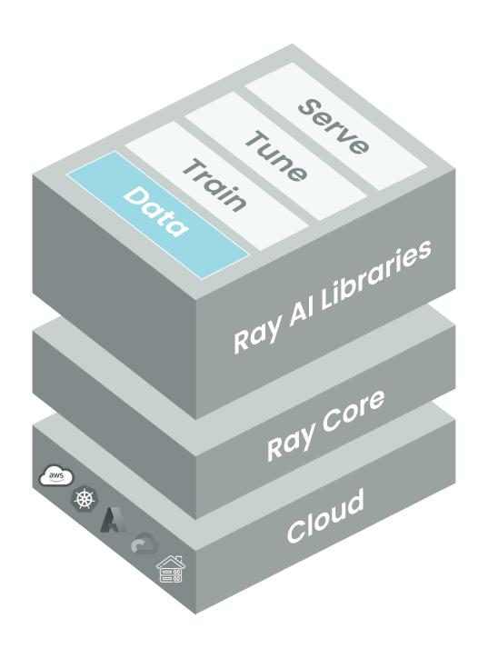
Ray-ai-libraries
Adding Ray Data for Distributed Data Processing
Optimize your data pipeline for ViT image classification using Ray Data in this notebook. The notebook covers topics like distributed data processing, creating a Ray Dataset, image preprocessing, setting up training logic, launching distributed fine-tuning, and performing batch inference with Ray Data.
3. Data Pipeline Optimization with Ray Data and Ray Train for ViT Image Classification
Milestone 3: Handling Big Data with Ray Data
Our previous notebook introduced Ray Train, enabling distributed training and resource efficiency. We’ve already fine-tuned our ViT model with enhanced scalability. Now, we’re poised to extend our work by optimizing our data pipeline with Ray Data.
In this notebook, we’ll replace the beans dataset with our own image data from S3 and use Ray Data for distributed data processing and you’ll see how it easily composes with Ray Train to scale these two MLOps stages.
Featured Libraries
- Ray Data
- A scalable data processing library for ML workloads that provides flexible and performant APIs for scaling batch inference and data preprocessing and ingest.
- Ray Train
- Hugging Face
transformers - Hugging Face
datasets
Table of Contents
- Introduction to Ray Data
- Distributed data processing for ML training and inference.
- Create a Ray Dataset
- Read new images from S3.
- Image Preprocessing
- Filter images.
- Featurize raw images.
- Set-Up Training Logic
- Prepare Hugging Face training logic for Ray Train.
- Launch Distributed Fine-Tuning
- Training at scale.
- Perform Batch Inference with Ray Data
- Load the fine-tuned model from the checkpoint to map to batches of new data.
1. Introduction to Ray Data
Data is the lifeblood of machine learning, and its efficient handling can significantly impact the training process. As datasets grow larger and more complex, managing data becomes increasingly challenging. This is especially true if the scaling solution for your data meets an opinionated scaling solution for training, and this manual stitching introduces a lot of operational overhead.
Here’s the cliffnotes introduction to Ray Data:
Efficient Data Loading: Ray Data offers tools and optimizations for efficient data loading, ensuring that data is readily available when needed, reducing training bottlenecks.
Parallel Data Processing: With Ray Data, we can easily parallelize data preprocessing, transforming, and augmentation, which is crucial for accelerating training and enhancing model performance.
Data Pipelines: Ray Data allows us to create data pipelines that seamlessly integrate with Ray Train, streamlining the entire machine learning workflow from ingest and preprocessing to batch inference.
2. Create a Ray Dataset
In the initial example, we used the beans dataset from Hugging Face, reading it in with their convenient load_dataset utility. Let’s now try our hand at working with some larger, messier data to demonstrate how you can use Ray Data for distributed ingest and processsing for your ML pipeline.
First, we must create a Ray Dataset, which is the standard way to load and exchange data in the Ray AI Libraries. Beginning with raw images of dogs and fish stored in S3, we’ll use read_images and union to generate this Ray Dataset.
Note: For the sake of time in class, we’re limiting the number of images retrieved, but feel free to experiment with the whole dataset.
import raydog_images_path = 's3://anonymous@air-example-data-2/imagenette2/train/n02102040'
fish_images_path = 's3://anonymous@air-example-data-2/imagenette2/train/n01440764'
ray_ds_images = ray.data.read_images(dog_images_path).limit(200).union(ray.data.read_images(fish_images_path).limit(200))Inspect a few images
ray_ds_images.schema()ray_ds_images.take(1)import PIL.Image
im = ray_ds_images.take(1)[0]['image']
PIL.Image.fromarray(im)Load labels
For this binary classification task, we’re distinguishing between images of dogs and images of fish. For this, we’ll need to fetch the ground truth labels, move those to shared storage, and load those (in this example, as a csv).
! cp /home/ray/default/ray-summit-2023-training/Ray_AI_Libraries/labels.csv /mnt/cluster_storage/labels.csvray_ds_labels = ray.data.read_csv('/mnt/shared_storage/summit_assets/labels.csv')Inspect a few labels
ray_ds_labels.schema()ray_ds_labels.take(4)Zip images and labels together
We can use zip to combine the data and labels.
labeled_ds = ray_ds_images.zip(ray_ds_labels)labeled_ds.schema()3. Image Preprocessing
Filtering wonky images
In real-world data, there are some problematic records. In this case, there are grayscale images without a proper 3rd axis in the image data tensor.
Let’s count them.
labeled_ds.map(lambda record:{'dims':record['image'].ndim}).groupby('dims').count().take_all()It’s a small number, so we can probably filter them out (there are statistical considerations to whether this is a useful move in general, but for us it will work).
filtered_labeled_ds = labeled_ds.filter(lambda record: record['image'].ndim==3)Featurize images
Much like we’ve done before, we need to use the associated ViT feature extractor to transform raw images to the format that the model expects. Applying this transformation is a great example of stateful transformation with Ray Data’s map_batches.
Note: You can also extend this general pattern for batch inference where you apply, a model for example, to batches of data to generate predictions.
from transformers import ViTImageProcessorclass Featurizer:
def __init__(self):
self._model_name_or_path = 'google/vit-base-patch16-224-in21k'
self._feature_extractor = ViTImageProcessor.from_pretrained(self._model_name_or_path)
def __call__(self, batch):
inputs = self._feature_extractor([x for x in batch['image']], return_tensors='pt')
return { 'pixel_values' : inputs['pixel_values'], 'labels' : batch['label'] }featurized_ds = filtered_labeled_ds.map_batches(Featurizer, compute=ray.data.ActorPoolStrategy(size=2))featurized_ds.schema()Create a train/test split
At this point, our dataset is more or less ready. Since we have a single labeled dataset, we’ll use train_test_split to create train/test subsets.
Note: this feature has some performance costs – we may want to avoid this, by externally producing training/validation/test sets where possible
train_dataset, valid_dataset = featurized_ds.train_test_split(test_size=0.2)4. Set-Up Training Logic
Everything below is the same, except for the following lines:
    train_sh = get_dataset_shard("train")
    training = train_sh.iter_torch_batches(batch_size=64)

    val_sh = get_dataset_shard("valid")
    valid = val_sh.iter_torch_batches(batch_size=64)
This fetches the DataIterator shard from a Ray Dataset and uses iter_torch_batches to convert to the type that our framework (Hugging Face) expects.
import torch
import numpy as np

from ray.train import ScalingConfig
from ray.train.torch import TorchTrainer
from ray.train.huggingface.transformers import prepare_trainer, RayTrainReportCallback
from transformers import ViTForImageClassification, TrainingArguments, Trainer, ViTImageProcessor
def train_func(config):
import evaluate
from ray.train import get_dataset_shard
train_sh = get_dataset_shard("train")
training = train_sh.iter_torch_batches(batch_size=64)
val_sh = get_dataset_shard("valid")
valid = val_sh.iter_torch_batches(batch_size=64)
labels = config['labels']
model = ViTForImageClassification.from_pretrained(config['model'], num_labels=len(labels))
metric = evaluate.load("accuracy")
def compute_metrics(eval_pred):
logits, labels = eval_pred
predictions = np.argmax(logits, axis=-1)
return metric.compute(predictions=predictions, references=labels)
# Hugging Face Training Args + Trainer
training_args = TrainingArguments(
output_dir="/mnt/cluster_storage/output",
evaluation_strategy="steps",
eval_steps = 3,
per_device_train_batch_size=128,
logging_steps=2,
save_steps=4,
max_steps=10,
)
trainer = Trainer(
model=model,
args=training_args,
compute_metrics=compute_metrics,
train_dataset=training,
eval_dataset=valid,
)
callback = RayTrainReportCallback()
trainer.add_callback(callback)
trainer = prepare_trainer(trainer)
trainer.train()5. Launch Distributed Fine-Tuning
This code is similar to the piece we encountered in the previous notebook with one small addition.
datasets here specifies the Ray Datasets we’ll be using in the training loop. Before, we loaded the Hugging Face datasets in the training function directly to avoid serialization errors when transferring the objects to the workers.
ray_trainer = TorchTrainer(
    train_loop_per_worker= train_func,
    train_loop_config= {'model':'google/vit-base-patch16-224-in21k', 'labels':ray_ds_labels.unique('label')},
    scaling_config=ScalingConfig(num_workers=2, use_gpu=True),
    run_config=ray.train.RunConfig(storage_path='/mnt/cluster_storage'),
    datasets={"train": train_dataset, "valid": valid_dataset},
)

result = ray_trainer.fit()
checkpoint_path = result.checkpoint.path6. Perform Batch Inference with Ray Data
Now that we have a fine-tuned model, let’s load it from the Ray Train checkpoint to generate some predictions on our test set. To do this, we’ll use Ray Data once again to load and featurize image batches and then apply the ViT model to generate predictions.
Load test set images
dog_test_images_path = 's3://anonymous@air-example-data-2/imagenette2/val/n02102040'
fish_test_images_path = 's3://anonymous@air-example-data-2/imagenette2/val/n01440764'

ray_ds_test_images = ray.data.read_images(dog_test_images_path, mode="RGB").limit(200).union(ray.data.read_images(fish_test_images_path, mode="RGB").limit(200))
Featurize images
suffix = '/checkpoint'
saved_model_path = checkpoint_path + suffix

BATCH_SIZE = 100 # Bump this up to the largest batch size that can fit on your GPUs
Using a class allows us to put the expensive pipeline loading and initialization code in the __init__ constructor, which will run only once. The actual model inference logic is in the __call__ method, which will be called for each batch.
The __call__ method takes a batch of data items, instead of a single one. In this case, the batch is a dict that has one key named “image”, and the value is a Numpy array of images represented in np.ndarray format.
from PIL import Imageclass ImageClassifier:
def __init__(self):
self._feature_extractor = ViTImageProcessor.from_pretrained('google/vit-base-patch16-224-in21k')
self._model = ViTForImageClassification.from_pretrained(saved_model_path)
self._model.eval()
def __call__(self, batch):
outputs = []
for image_array in batch["image"]:
image = Image.fromarray(image_array)
input = self._feature_extractor(image, return_tensors='pt')
output = self._model(input['pixel_values']).logits.numpy(force=True)
outputs.append(output)
return {'results': outputs}
We use the map_batches API to apply the model to the whole dataset.
The first parameter of map_batches is the user-defined function (UDF), which can either be a function or a class. Since we are using a class in this case, the UDF will run as long-running Ray actors. For class-based UDFs, we use the compute argument to specify ActorPoolStrategy with the number of parallel actors. And the batch_size argument indicates the number of images in each batch.
The num_gpus argument specifies the number of GPUs needed for each ImageClassifier instance. In this case, we want 1 GPU for each model replica.
predictions = ray_ds_test_images.map_batches(
    ImageClassifier,
    compute=ray.data.ActorPoolStrategy(size=2), # Use 2 GPUs. Change this number based on the number of GPUs in your cluster.
    num_gpus=1,  # Specify 1 GPU per model replica.
    batch_size=BATCH_SIZE # Use the largest batch size that can fit on our GPUs
)predictions.take_batch(5)