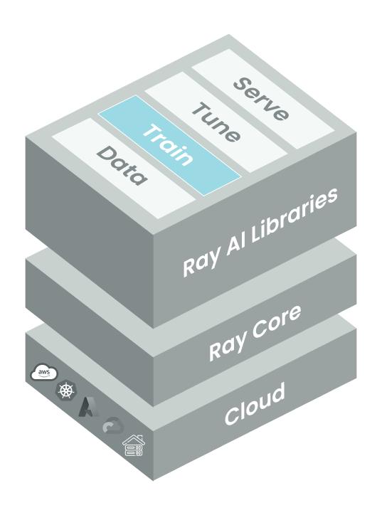
Ray-ai-libraries
Adding Ray Train for Distributed Fine-tuning
Leverage the power of Ray Train for distributed machine learning training in this notebook focused on ViT image classification. Explore the capabilities of Ray Train, which enables distributed training and efficient resource utilization.
2. Scalable Training with Ray Train for ViT Image Classification
Milestone 2: Distributed ML Training with Ray Train
In this notebook, we’ll adapt our initial example to leverage Ray Train, a powerful library that enables distributed training and efficient utilization of resources. This transformation marks the beginning of our journey toward building scalable machine learning pipelines with Ray.
Featured Libraries
- Ray Train
- Built on top of Ray, it’s a scalable machine learning library for distributed training and fine-tuning.
- Hugging Face
transformers - Hugging Face
datasets
Table of Contents
- Introduction to Ray Train
- What is Ray Train and what kinds of problems does it solve?
- Define the Training Logic
- Create a
train_functhat will be executed on each distributed training worker.
- Create a
- Configure the Scale and GPUs
- Move from a laptop to a cluster in the cloud with ease and control.
- Learn how to make the most of multiple GPUs using Ray Train, speeding up training by parallelizing computations.
- Launch Distributed Fine-Tuning
- Explore how Ray Train enables efficient data parallelism, distributing the data across multiple workers for faster training.
- Access Training Results
- Inspect the final output.
1. Introduction to Ray Train
Before we dive into the technical details, let’s briefly understand why we’re using Ray Train:
Scalability: Ray Train allows us to easily distribute training across multiple GPUs and different machines, making it possible to handle large datasets and complex models efficiently.
Resource Efficiency: With Ray Train, we can maximize the use of available resources, ensuring that our fine-tuning process is not bottlenecked by hardware limitations.
Flexibility: It seamlessly integrates with popular existing machine learning libraries like the PyTorch ecosystem, Tensorflow, XGBoost, and more, making it straightforward to adapt your existing workflows.
Building on our foundation
Our previous notebook laid the groundwork for this transition. We’re already familiar with the components like that dataset, feature extractor, model, and training logic. Let’s see how we can adapt that existing code to now leverage the capabilities of Ray Train.
2. Define the Training Logic
To give you a sense of the shape of the final implementation, here’s the pattern we’re trying to achieve:
from ray.train.torch import TorchTrainer
from ray.train import ScalingConfig

def train_func(config):
    # Your Transformers training code here.

scaling_config = ScalingConfig(num_workers=2, use_gpu=True)
trainer = TorchTrainer(train_func, scaling_config=scaling_config)
result = trainer.fit()
In the following section, we’ll implement each of these steps in detail:
train_func- Wraps all of your existing training logic and will be executed on each distributed training worker.ScalingConfig- Specifies the number of workers and computing resources to use for each.TorchTrainer- Launches the distributed training job.
Imports
import torch
import numpy as np
import ray.train.huggingface.transformers


from ray.train import ScalingConfig
from ray.train.huggingface.transformers import prepare_trainer, RayTrainReportCallback
from ray.train.torch import TorchTrainer
from transformers import ViTForImageClassification, TrainingArguments, Trainer, ViTImageProcessor
Wrap training logic in a train_func
We’ll take the essense of the previous notebook and distill is in the most compact way in this training function.
Note: You’ll see here that we’re loading the dataset, feature extractor, and model within this function which will be replicated across every worker. This pattern may not be ideal for large datasets and models, and we’ll explore how to deal with this in the next notebook.
def train_func(config):
    from datasets import load_dataset
    import evaluate

    # HF dataset
    ds = load_dataset('beans')

    # HF feature extractor
    model_name_or_path = 'google/vit-base-patch16-224-in21k'
    feature_extractor = ViTImageProcessor.from_pretrained(model_name_or_path)

    # HF ViT model
    labels = ds['train'].features['labels'].names
    model = ViTForImageClassification.from_pretrained(
        model_name_or_path,
        num_labels=len(labels),
        id2label={str(i): c for i, c in enumerate(labels)},
        label2id={c: str(i) for i, c in enumerate(labels)}
    )

    # Image processing
    def transform(example_batch):
        inputs = feature_extractor([x for x in example_batch['image']], return_tensors='pt')
        inputs['labels'] = example_batch['labels']
        return inputs

    prepared_ds = ds.with_transform(transform)

    # Evaluation metric
    metric = evaluate.load("accuracy")

    def compute_metrics(eval_pred):
        logits, labels = eval_pred
        predictions = np.argmax(logits, axis=-1)
        return metric.compute(predictions=predictions, references=labels)

    # HF Training Args
    training_args = TrainingArguments(
      output_dir="/mnt/local_storage/output",
      evaluation_strategy="steps",
      eval_steps = 3,
      num_train_epochs=2,
      logging_steps=2,
      save_steps=4,
      max_steps=10,
      remove_unused_columns=False,
    )

    # Data collector
    def collate_fn(batch):
        return {
            'pixel_values': torch.stack([x['pixel_values'] for x in batch]),
            'labels': torch.tensor([x['labels'] for x in batch])
        }

    # HF Trainer
    trainer = Trainer(
        model=model,
        args=training_args,
        data_collator=collate_fn,
        compute_metrics=compute_metrics,
        train_dataset=prepared_ds["train"],
        eval_dataset=prepared_ds["validation"],
    )

    # Report metrics and checkpoints to Ray Train
    callback = RayTrainReportCallback()
    trainer.add_callback(callback)

    # Prepare transformers Trainer for Ray Train; enables Ray Data integration.
    trainer = prepare_trainer(trainer)

    # Start training
    trainer.train()
3. Configure the Scale and GPUs
Define a ScalingConfig
Today, we have access to two workers, each with access to 1 GPU, so we’ll set the ScalingConfig to match. With more or varied resources, you’re able to have greater freedom in specifying not only a larger cluster, but heterogeneous and custom hardware.
num_workers- The number of distributed training worker processes.use_gpu- Whether each worker should use a GPU (or CPU).
scaling_config = ScalingConfig(num_workers=2, use_gpu=True)Create a Ray Train TorchTrainer
Note: While I won’t cover the RunConfig in great detail, know that it allows you to set things like the experiment name, storage path for results, stopping conditions, custom callbacks, checkpoint configuration, verbosity level, and logging options.
ray_trainer = TorchTrainer(
    train_func, scaling_config=scaling_config,
    run_config=ray.train.RunConfig(storage_path='/mnt/cluster_storage')
)
4. Launch Distributed Fine-Tuning
result = ray_trainer.fit()5. Access Training Results
Once this job completes, you’ll be able to access a Result object which contains more information about the training run, including the metrics and checkpoints reported during training.
result.metrics     # The metrics reported during training.
result.checkpoint  # The latest checkpoint reported during training.
result.path        # The path where logs are stored.
result.error # The exception that was raised, if training failed.print(result.metrics)