Ray-ai-libraries
Plain Hugging Face Image Classification
While this notebook focuses on using Hugging Face without Ray, it sets the foundation for subsequent notebooks, where Ray Train, Ray Data, and Ray Serve will be introduced for scalable machine learning. Explore the basics of fine-tuning ViTs for image classification, building a strong starting point for more advanced tasks in the following notebooks.
1. Fine-Tune ViT for Image Classification with Hugging Face
Milestone 1: Using Plain Hugging Face Transformers
In this kick-off notebook, we’re jumping straight into one of the most active areas of deep learning: transformers. You’ve likely heard of using transformers for natural language tasks, but there’s also been great strides in using this architecture for audio, visual, and other multimodal applications. Today we’ll be fine-tuning Vision Transformers (ViTs) for image classification using Hugging Face, without Ray.
But, this isn’t just a one-and-done exercise! This initial example serves as the foundation for our subsequent notebooks, where we’ll gently weave in the capabilities of Ray Train, Ray Data, and Ray Serve for scalable machine learning. So, let’s get familiar with the base logic here so that we can hit the ground running in the next notebook.
Credit: This notebook is based on Nate Raw’s blog “Fine-Tune ViT for Image Classification with 🤗 Transformers”.
Featured Libraries
- Hugging Face
transformers- A popular library for working with transformer models, which we will use for accessing and fine-tuning a pretrained Vision Transformer.
- Hugging Face
datasets- Useful for accessing and sharing datasets with the larger AI community; usually much cleaner than real-world data.
Table of Contents
- Set-Up
- Load the dataset
- Load the feature extractor
- Load the model
- Image Processing
- Establish Training Logic
- Define data collector
- Define evaluation metric
- Define training arguments
- Launch Fine-Tuning
1. Set-up
The Vision Transformer, or ViT for short, was introduced in a groundbreaking paper by researchers at Google Brain in June 2021. This innovation explores the concept of tokenizing images, similar to how we tokenize sentences in NLP, enabling us to leverage transformer models for image-related tasks.
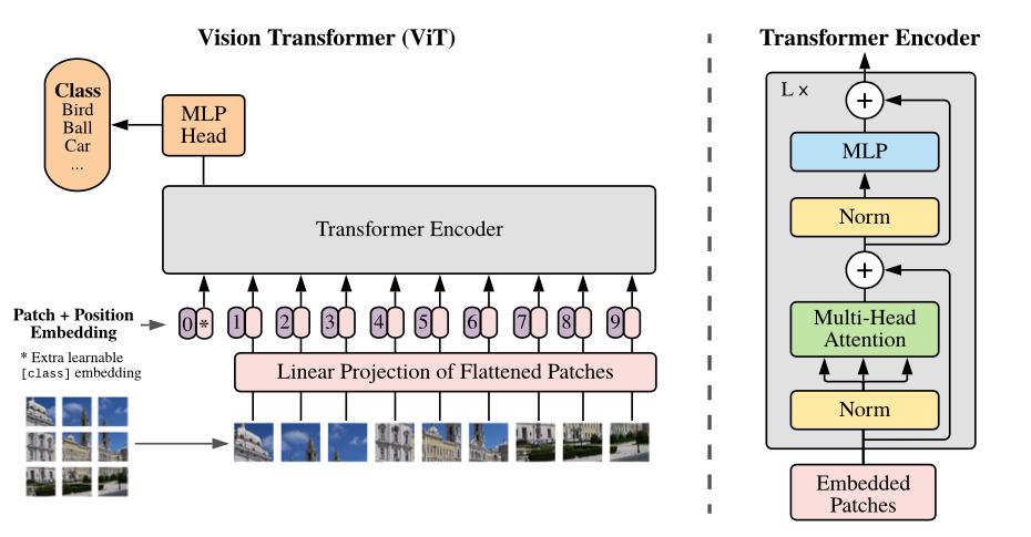
This approach can be summarized in three major steps:
Image Tokenization: Images are divided into a grid of sub-image patches.
Linear Projection: Each patch is embedded using a linear projection, effectively converting visual content into numerical representations.
Tokenized Sequence: These embedded patches are treated as tokens, forming a sequence that can be processed by transformer models.
Imports
As mentioned above, the focus areas here will be using Hugging Face’s datasets and transformers libraries to fine-tune our Vision Transformer.
import torch
import numpy as np

from datasets import load_dataset, load_metric
from transformers import ViTFeatureExtractor, ViTForImageClassification, TrainingArguments, Trainer
Load the Hugging Face dataset
For ease of start-up, we’ll use the beans dataset which contains ~1000 images of bean leaves with the intention of classifying healthy and diseased plants.
Note: Later on, we’ll replace this dataset a form you’ll likely encounter in a real pipeline, like reading from an S3 bucket.
ds = load_dataset('beans', cache_dir='/mnt/local_storage')Load the ViT feature extractor
Each Hugging Face transformer model has an associated FeatureExtractor which crystallizes the logic for transforming raw data into a format suited for that particular model.
model_name_or_path = 'google/vit-base-patch16-224-in21k'
feature_extractor = ViTFeatureExtractor.from_pretrained(model_name_or_path)
Load the ViT model
We’ll fetch the pretrained model from the Hugging Face Hub, and importantly, specify num_labels to set the correct dimensions for the classification head (should be 2 for binary classification).
The mapping of id2label and label2id just translates between indices and human-readable labels
labels = ds['train'].features['labels'].names

model = ViTForImageClassification.from_pretrained(
    model_name_or_path,
    num_labels=len(labels),
    id2label={str(i): c for i, c in enumerate(labels)},
    label2id={c: str(i) for i, c in enumerate(labels)}
)
2. Image Processing
With the feature extractor we loaded, let’s transform the beans dataset in preparation for training.
def transform(example_batch):
    # Take a list of PIL images and turn them to pixel values as torch tensors.
    inputs = feature_extractor([x for x in example_batch['image']], return_tensors='pt')

    # Don't forget to include the labels!
    inputs['labels'] = example_batch['labels']
    return inputs
prepared_ds = ds.with_transform(transform)3. Establish Training Logic
In this section, we’ll prepare all of the necessary logic to feed into the Hugging Face Trainer that executes our fine-tuning step.
Define the data collector
This collate function unpacks and stacks batches from lists of dicts to batch tensors.
def collate_fn(batch):
    return {
        'pixel_values': torch.stack([x['pixel_values'] for x in batch]),
        'labels': torch.tensor([x['labels'] for x in batch])
    }
Define an evaluation metric
With a classification task, we can just compare the ground truth labels with the predictions to get a first-order evaluation metric.
metric = load_metric("accuracy")

def compute_metrics(p):
    return metric.compute(predictions=np.argmax(p.predictions, axis=1), references=p.label_ids)
Set-up TrainingArguments
In the transformers library, you can specify a variety of hyperparameters, optimizers, and other options in your TrainingArguments configuration. One to call out here is remove_unused_columns=False which preserves our “unused” image because it is necessary for generating pixel values.
training_args = TrainingArguments(
  output_dir="/mnt/local_storage/vit-base-beans-demo-v5",
  per_device_train_batch_size=16,
  evaluation_strategy="steps",
  num_train_epochs=4,
  fp16=True,
  save_steps=100,
  eval_steps=100,
  logging_steps=10,
  learning_rate=2e-4,
  save_total_limit=2,
  remove_unused_columns=False,
  push_to_hub=False,
  report_to='tensorboard',
  load_best_model_at_end=True,
)
Construct the Trainer
trainer = Trainer(
    model=model,
    args=training_args,
    data_collator=collate_fn,
    compute_metrics=compute_metrics,
    train_dataset=prepared_ds["train"],
    eval_dataset=prepared_ds["validation"],
    tokenizer=feature_extractor,
)
4. Launch Fine-Tuning
train_results = trainer.train()

trainer.save_model()
trainer.log_metrics("train", train_results.metrics)
trainer.save_metrics("train", train_results.metrics)
trainer.save_state()
Alright, now that we have the basic flow, let’s go to the next notebook to see how to adapt the fine-tuning step with Ray Train to take advantage of a cluster!